Python Parkinson's Classification

Parkinson's Detection

9 minute read

Part 1 - INTRODUCTION

Parkinson’s disease is a brain disorder that causes unintended or uncontrollable movements, such as shaking, stiffness, and difficulty with balance and coordination.

Symptoms usually begin gradually and worsen over time. As the disease progresses, people may have difficulty walking and talking.

While virtually anyone could be at risk for developing Parkinson’s, some research studies suggest this disease affects more men than women. It’s unclear why, but studies are underway to understand factors that may increase a person’s risk. One clear risk is age: Although most people with Parkinson’s first develop the disease after age 60, about 5% to 10% experience onset before the age of 50. Early-onset forms of Parkinson’s are often, but not always, inherited, and some forms have been linked to specific gene mutations.

More than 10 million people worldwide are affected by Parkinson’s Disease in present day. Since there is no known cure for Parkinson’s, doctors are collecting data to identify the disease earlier and develop better treatments or potential cures. In this analysis, I will use a set of patient data to predict a patient’s likelihood of having Parkinson’s Disease via several machine learning models.

—- Results —-

After running several different models on the data, I determined that a random forest model was best able to predict Parkinson’s Disease with an accuracy of 100% and F1 score of 100%.

—- Data Source and Notes —-

Data source: https://www.kaggle.com/datasets/nidaguler/parkinsons-data-set

Data column dictionary:

name - ASCII subject name and recording number
MDVP:Fo(Hz) - Average vocal fundamental frequency
MDVP:Fhi(Hz) - Maximum vocal fundamental frequency
MDVP:Flo(Hz) - Minimum vocal fundamental frequency
MDVP:Jitter(%),MDVP:Jitter(Abs),MDVP:RAP,MDVP:PPQ,Jitter:DDP - Several
measures of variation in fundamental frequency
MDVP:Shimmer,MDVP:Shimmer(dB),Shimmer:APQ3,Shimmer:APQ5,MDVP:APQ,Shimmer:DDA - Several measures of variation in amplitude
NHR,HNR - Two measures of ratio of noise to tonal components in the voice
status - Health status of the subject (one) - Parkinson’s, (zero) - healthy
RPDE,D2 - Two nonlinear dynamical complexity measures
DFA - Signal fractal scaling exponent
spread1,spread2,PPE - Three nonlinear measures of fundamental frequency variation

—- Import Libraries for Project —-

import pandas as pd
import numpy as np
import matplotlib.pyplot as plt
from sklearn.ensemble import RandomForestClassifier
from sklearn.utils import shuffle
from sklearn.model_selection import train_test_split
from sklearn.metrics import confusion_matrix,plot_confusion_matrix,accuracy_score,precision_score,recall_score,f1_score
from sklearn.preprocessing import OneHotEncoder,MinMaxScaler
from sklearn.inspection import permutation_importance

from sklearn.neighbors import KNeighborsClassifier
from sklearn.feature_selection import RFECV

from sklearn.linear_model import LogisticRegression

Part 2 - Data Preparation and Exploration

First, the Parkinson’s dataset is loaded. This data was gathered from Kaggle (https://www.kaggle.com/nidaguler/parkinsons-data-set).

data = pd.read_csv('../input/parkinsons-data-set/parkinsons.data')

Prepare Data

The dataset used for this project, provided by Max Little of Oxford, was cleaned/formatted prior to it being posted on Kaggle for public use. Luckily, that means all we have to do is drop the ‘name’ column since it only contains unique identifiers/keys. This is done in the next section.

Perform EDA

First, we can drop the ‘name’ column as mentioned above.

data.drop('name',axis=1,inplace=True)

Next, we can get the head of the data to see the general data formatting and structure

data.head()

From the head call, we see that there are 24 columns and each of them is numeric. Glancing quickly at the columns we can see the columns are not all on the same scale, so some scaling will need to take place before analysis can occur.

We can also look to see if there are any null values in our data.

data.info()

The info call shows that each column has 195 non-null values, so there is no need to analyze further for rows with incomplete data.

Before splitting the data for analysis, we want to make sure the data is shuffled. If the data was ordered in a particular way to start, shuffling will help ensure that the train/test data sets are more likely to be representative of the whole data set.

data = shuffle(data,random_state=42)

As noted by the original authors, many of the people tested had Parkinson’s disease. We want to make sure that our data isn’t too imbalanced, or else further data preparation may be needed to account for such imbalance. We do this by determining the percent of recordings that had a positive status for Parkinson’s Disease.

data['status'].value_counts(normalize=True) 

Running the above code, we find that 75% of rows have a positive status. Though this indicates that there are more positive instances, there should be enough instances of both positive and negative results to continue with the analysis without further preparation.

—- Hypothesize a Solution —-

In the next parts of this analysis, I will attempt to classify the given data points and predict whether a given patient has Parkinson’s. To do so, I will test three models:

KNN Classifier
Random Forest Classifier
Logistic Regression Classifier

Part 3 - Develop A Model

First I will split the data into an X feature group and y target class group, and further split into a train and test set.

X=data.drop('status',axis=1)
y=data['status']

X_train, X_test, y_train, y_test = train_test_split(X, y, test_size=0.2, random_state=42)

Logistic Regression Classifier Model

With the above step taken, I can now train a model to predict Parkinson’s Disease likehlihood. I will first train a Logistic model as a baseline. To do so, I will scale the data, determine the optimal number of features to use, and then fit a model to the resulting processed dataset.

scaler = MinMaxScaler()

X_train_lr = pd.DataFrame(scaler.fit_transform(X_train),columns=X_train.columns) #return as df
X_test_lr = pd.DataFrame(scaler.transform(X_test),columns=X_test.columns) #return as df

clf_lr = LogisticRegression(random_state=42,max_iter=1000)

feature_selector = RFECV(clf_lr, cv=5)

fit=feature_selector.fit(X_train,y_train)

optimal_feature_count = feature_selector.n_features_
print(f'the optimal number of features is: {optimal_feature_count}')

X_train_lr = X_train_lr.loc[:,feature_selector.get_support()]
X_test_lr = X_test_lr.loc[:,feature_selector.get_support()]

#understand how much better it is to have 2 vars than any other #

plt.plot(range(1,len(fit.grid_scores_)+1),fit.grid_scores_,marker='o')
#range used so x axis goes from 1 to 4 features rather than starting at 0
#second fit is the scores for each number of vars
plt.ylabel("model score")
plt.xlabel('number of features')
plt.title(f'Feature Selection using RFE \n Optimal number of features is {optimal_feature_count} (at score of {round(max(fit.grid_scores_),3)})')
plt.tight_layout()
plt.show()

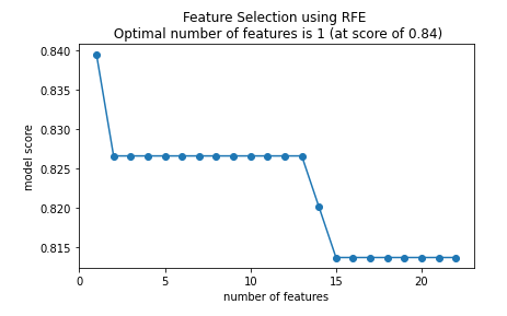
As shown above, it appears that the optimal number of features to use is 1.

clf=LogisticRegression(random_state=42,max_iter=1000)
clf.fit(X_train_lr,y_train)

y_pred_class = clf.predict(X_test_lr)
y_pred_proba = clf.predict_proba(X_test_lr)[:,1]

confusion_matrix(y_test, y_pred_class)

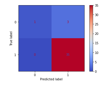
plot_confusion_matrix(clf,X_test_lr,y_test,cmap='coolwarm')

#Accuracy ((# of correct classifactions out of all attempted classifications))

accuracy_score(y_test,y_pred_class)

# Precision (of all observations that were predicted +, how many were actually +)
precision_score(y_test,y_pred_class)

#Recall (of all + observations, how many did we predict as +)
recall_score(y_test,y_pred_class)

#f1 score (harmonic mean of recall and precision)
f1_score(y_test,y_pred_class)

After running the above Logistic model, we get a result with an F1 score of 95.9%! This model appears to predict Parkinson’s well for patients in this dataset. I would still like to run a few more models to see if any improvements can be made.

KNN Model

Next, I will train a KNN model on the patient data.

data.describe()

Similar to the Logistic model, I will first scale my data, determine the optimal number of features to use in the model, and then train a model on the data.

scaler = MinMaxScaler()

X_train_knn = pd.DataFrame(scaler.fit_transform(X_train),columns=X_train.columns) #return as df
X_test_knn = pd.DataFrame(scaler.transform(X_test),columns=X_test.columns) #return as df

from sklearn.ensemble import RandomForestClassifier


clf = RandomForestClassifier(random_state=42)

feature_selector = RFECV(clf, cv=5)

fit=feature_selector.fit(X_train_knn,y_train)

optimal_feature_count = feature_selector.n_features_
print(f'the optimal number of features is: {optimal_feature_count}')

X_train_knn = X_train_knn.loc[:,feature_selector.get_support()]
X_test_knn = X_test_knn.loc[:,feature_selector.get_support()]

#understand how much better it is to have 2 vars than any other #

plt.plot(range(1,len(fit.grid_scores_)+1),fit.grid_scores_,marker='o')
#range used so x axis goes from 1 to 4 features rather than starting at 0
#second fit is the scores for each number of vars
plt.ylabel("model score")
plt.xlabel('number of features')
plt.title(f'Feature Selection using RFE \n Optimal number of features is {optimal_feature_count} (at score of {round(max(fit.grid_scores_),3)})')
plt.tight_layout()
plt.show()

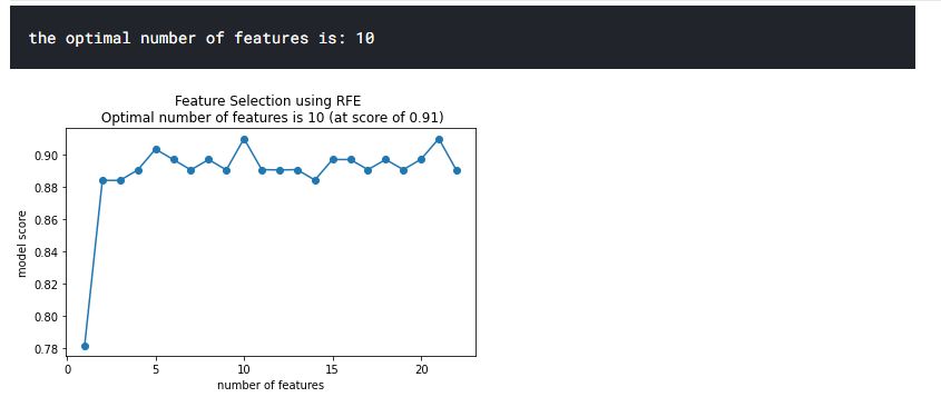
As shown above, the optimal number of features to use for this model is 10.

Now I will train a KNN model on the data.

clf=KNeighborsClassifier()
clf.fit(X_train_knn,y_train)

y_pred_class = clf.predict(X_test_knn)
y_pred_proba = clf.predict_proba(X_test_knn)[:,1]


confusion_matrix(y_test, y_pred_class)

plot_confusion_matrix(clf,X_test_knn,y_test,cmap='coolwarm')

#Accuracy ((# of correct classifactions out of all attempted classifications))

accuracy_score(y_test,y_pred_class)

# Precision (of all observations that were predicted +, how many were actually +)
precision_score(y_test,y_pred_class)

#Recall (of all + observations, how many did we predict as +)
recall_score(y_test,y_pred_class)

#f1 score (harmonic mean of recall and precision)
f1_score(y_test,y_pred_class)

The above analysis shows that this model has an F1 score of 97.1%, slightly worse than the Logistic model.

I would like to know what the optimal number for K is, for potential future work and analysis. To do so, I will run a KNN model for a range of K values.

k_list = list(range(2,25))

accuracy_scores= []
for k in k_list:
    clf= KNeighborsClassifier(n_neighbors=k)
    clf.fit(X_train_knn,y_train)
    y_pred=clf.predict(X_test_knn)
    accuracy = f1_score(y_test,y_pred)
    accuracy_scores.append(accuracy)

max_accuracy = max(accuracy_scores)
max_accuracy_idx = accuracy_scores.index(max_accuracy)
optimal_k_value = k_list[max_accuracy_idx]

#plot of max depths

plt.plot(k_list,accuracy_scores)
plt.scatter(optimal_k_value,max_accuracy,marker='x',color='red')
plt.title(f"Accuracy (F1 Score) by K \n Optimal Value for K: {optimal_k_value} (Accuracy: {round(max_accuracy,4)})")
plt.xlabel('k')
plt.ylabel('accuracy (F1 Score)')
plt.tight_layout()
plt.show()

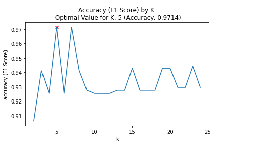
The above analysis shows that the optimal number for K is 5.

Random Forest Classification Analysis

The last model I will run is a random forest model, since these tend to run well on classification tasks.

I will not need to scale my data for this type of model, so I can jump right into training and testing:

clf=RandomForestClassifier(random_state=42,n_estimators=500,max_features=5)
clf.fit(X_train,y_train)

y_pred_class = clf.predict(X_test)
y_pred_proba = clf.predict_proba(X_test)[:,1]

confusion_matrix(y_test, y_pred_class)

plot_confusion_matrix(clf,X_test,y_test,cmap='coolwarm')

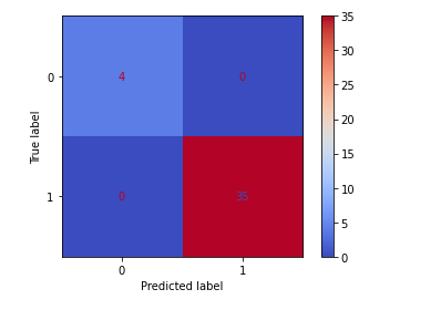
accuracy_score(y_test,y_pred_class)
# 1.0

precision_score(y_test,y_pred_class)
# 1.0

recall_score(y_test,y_pred_class)
# 1.0

f1_score(y_test,y_pred_class)
# 1.0

The above analysis shows that the Random Forest model has an F1 score of 100%, beating out the original Logistic model’s results!

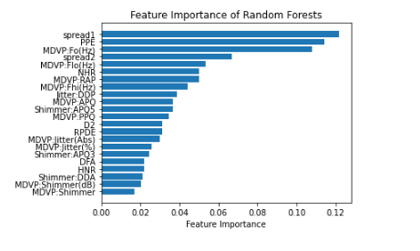
With this in mind, I also want to run a feature importance analysis to determine which features the Random Forest determined to be most important for classification.

feature_importance=pd.DataFrame(clf.feature_importances_)
feature_names=pd.DataFrame(X.columns)
feature_importance_summary = pd.concat([feature_names,feature_importance],axis=1)
feature_importance_summary.columns = ['input_variable','feature_importance']
feature_importance_summary.sort_values(by='feature_importance', inplace=True)

plt.barh(feature_importance_summary['input_variable'],feature_importance_summary['feature_importance'])
plt.title("Feature Importance of Random Forests")
plt.xlabel("Feature Importance")
plt.tight_layout()
plt.show()

result = permutation_importance(clf,X_test, y_test, n_repeats=10,random_state=42)
print(result)


permutation_importance=pd.DataFrame(result['importances_mean'])
feature_names=pd.DataFrame(X.columns)
permutation_importance_summary = pd.concat([feature_names,permutation_importance],axis=1)
permutation_importance_summary.columns = ['input_variable','permutation_importance']
permutation_importance_summary.sort_values(by='permutation_importance', inplace=True)

plt.barh(permutation_importance_summary['input_variable'],permutation_importance_summary['permutation_importance'])
plt.title("Permutation Importance of Random Forests")
plt.xlabel("Permutation Importance")
plt.tight_layout()
plt.show()

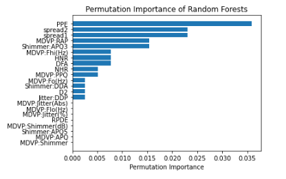
In the above feature and permutation importance charts, it appears that Spraed 1, Spread 2 and PPE are consistently shown as highly important.

Part 4 - POTENTIAL FUTURE WORK

In the future, it would be interesting to conduct more analysis to build on the current model.

For example, the random forest model permutation importance analysis showed that there were several features that were more prominent than others including PPE, Spread 1, and Spread 2. It would be interesting to hone in on these variables to create new measures/variables. Similarly, groups could study how these variables lead to increased Parkinson’s risk and further help doctors diagnose and prevent the disease in the future.

It would also be interesting to test this model out on a larger data set or find data sets with additional fields to classify on. This data set is relatively small, and I would want to make sure that it generalizes well in larger data sets as well.

Part 5 - CONCLUSION

Parkinson’s disease is a brain disorder that causes unintended or uncontrollable movements, such as shaking, stiffness, and difficulty with balance and coordination. More than 10 million people worldwide are affected by Parkinson’s Disease in present day.

In this analysis, I took a set of patient data with the goal of using it to predict a patient’s likelihood for having Parkinson’s so that they can be treated and have better quality of life overall.

To do this, I first analyzed whether the provided data was clean. Luckily, the original data uploader ensured that this data was of high fidelity.

Next, I split the data into test/train sets and ran three different models on the test/train data to see which performed best.

In the end, the random forest model performed best with accuracy of 100% and F1 score of 100%. Though this is great for the data I have, the provided data set is relatively small so I would like to test it on more instances and verify that the model generalizes well.

Allan Khariton

Data Science Portfolio